How to Train and Deploy a Linear Regression Model Using PyTorch – Part 1

Python is one of today’s most popular programming languages and is used in many different applications. The 2021 StackOverflow Developer Survey showed that Python remains the third most popular programming language among developers. In GitHub’s 2021 State of the Octoverse report, Python took the silver medal behind Javascript.

Thanks to its longstanding popularity, developers have built many popular Python frameworks and libraries like Flask, Django, and FastAPI for web development.

However, Python isn’t just for web development. It powers libraries and frameworks like NumPy (Numerical Python), Matplotlib, scikit-learn, PyTorch, and others which are pivotal in engineering and machine learning. Python is arguably the top language for AI, machine learning, and data science development. For deep learning (DL), leading frameworks like TensorFlow, PyTorch, and Keras are Python-friendly.

We’ll introduce PyTorch and how to use it for a simple problem like linear regression. We’ll also provide a simple way to containerize your application. Also, keep an eye out for Part 2 — where we’ll dive deeply into a real-world problem and deployment via containers. Let’s get started.

What is PyTorch?

A Brief History and Evolution of PyTorch

Torch debuted in 2002 as a deep-learning library developed in the Lua language. Accordingly, Soumith Chintala and Adam Paszke (both from Meta) developed PyTorch in 2016 and based it on the Torch library. Since then, developers have flocked to it. PyTorch was the third-most-popular framework per the 2021 StackOverflow Developer Survey. However, it’s the most loved DL library among developers and ranks third in popularity. Pytorch is also the DL framework of choice for Tesla, Uber, Microsoft, and over 7,300 others.

PyTorch enables tensor computation with GPU acceleration, plus deep neural networks built on a tape-based autograd system. We’ll briefly break these terms down, in case you’ve just started learning about these technologies.

• A tensor, in a machine learning context, refers to an n-dimensional array.
• A tape-based autograd means that Pytorch uses reverse-mode automatic differentiation, which is a mathematical technique to compute derivatives (or gradients) effectively using a computer.

Since diving into these mathematics might take too much time, check out these links for more information:

• What is a Pytorch Tensor?
• What is a tape-based autograd system?
• Automatic differentiation

PyTorch is a vast library and contains plenty of features for various deep learning applications. To get started, let’s evaluate a use case like linear regression.

What is Linear Regression?

Linear Regression is one of the most commonly used mathematical modeling techniques. It models a linear relationship between two variables. This technique helps determine correlations between two variables — or determines the value-dependent variable based on a particular value of the independent variable.

In machine learning, linear regression often applies to prediction and forecasting applications. You can solve it analytically, typically without needing any DL framework. However, this is a good way to understand the PyTorch framework and kick off some analytical problem-solving.

Numerous books and web resources address the theory of linear regression. We’ll cover just enough theory to help you implement the model. We’ll also explain some key terms. If you want to explore further, check out the useful resources at the end of this section.

Linear Regression Model

You can represent a basic linear regression model with the following equation:

Y = mX + bias

What does each portion represent?

• Y is the dependent variable, also called a target or a label.
• X is the independent variable, also called a feature(s) or co-variate(s).
• bias is also called offset.
• m refers to the weight or “slope.”

These terms are often interchangeable. The dependent and independent variables can be scalars or tensors.

The goal of the linear regression is to choose weights and biases so that any prediction for a new data point — based on the existing dataset — yields the lowest error rate. In simpler terms, linear regression is finding the best possible curve (line, in this case) to match your data distribution.

Loss Function

A loss function is an error function that expresses the error (or loss) between real and predicted values. A very popular way to measure loss is by using a root mean squared error, which we’ll also use.

Gradient Descent Algorithms

Gradient descent is a class of optimization algorithms that tries to solve the problem (either analytically or using deep learning models) by starting from an initial guess of weights and bias. It then iteratively reduces errors by updating weights and bias values with successively better guesses.

A simplified approach uses the derivative of the loss function and minimizes the loss. The derivative is the slope of the mathematical curve, and we’re attempting to reach the bottom of it — hence the name gradient descent. The stochastic gradient method samples smaller batches of data to compute updates which are computationally better than passing the entire dataset at each iteration.

To learn more about this theory, the following resources are helpful:

• MIT lecture on Linear regression
• Linear regression Wikipedia article
• Dive into deep learning online resources on linear regression

Linear Regression with Pytorch

Now, let’s talk about implementing a linear regression model using PyTorch. The script shown in the steps below is main.py — which resides in the GitHub repository and is forked from the “Dive Into Deep learning” example repository. You can find code samples within the pytorch directory.

For our regression example, you’ll need the following:

• Python 3
• PyTorch module (pip install torch) installed on your system
• NumPy module (pip install numpy) installed
• Optionally, an editor (VS Code is used in our example)

Problem Statement

As mentioned previously, linear regression is analytically solvable. We’re using deep learning to solve this problem since it helps you quickly get started and easily check the validity of your training data. This compares your training data against the data set.

We’ll attempt the following using Python and PyTorch:

• Creating synthetic data where we’re aware of weights and bias
• Using the PyTorch framework and built-in functions for tensor operations, dataset loading, model definition, and training

We don’t need a validation set for this example since we already have the ground truth. We’d assess our results by measuring the error against the weights and bias values used while creating our synthetic data.

Step 1: Import Libraries and Namespaces

For our simple linear regression, we’ll import the torch library in Python. We’ll also add some specific namespaces from our torch import. This helps create cleaner code:

# Step 1 import libraries and namespaces

import torch

from torch.utils import data

# `nn` is an abbreviation for neural networks

from torch import nn

Step 2: Create a Dataset

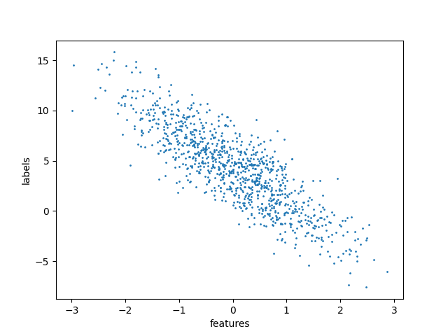
For simplicity’s sake, this example creates a synthetic dataset that aims to form a linear relationship between two variables with some bias.

i.e. y = mx + bias + noise

#Step 2: Create Dataset

#Define a function to generate noisy data

def synthetic_data(m, c, num_examples):

"""Generate y = mX + bias(c) + noise"""

X = torch.normal(0, 1, (num_examples, len(m)))

y = torch.matmul(X, m) + c

y += torch.normal(0, 0.01, y.shape)

return X, y.reshape((-1, 1))

 

true_m = torch.tensor([2, -3.4])

true_c = 4.2

features, labels = synthetic_data(true_m, true_c, 1000)

Here, we use the built-in PyTorch function torch.normal to return a tensor of normally distributed random numbers. We’re also using the torch.matmul function to multiply tensor X with tensor m, and Y is distributed normally again.

The dataset looks like this when visualized using a simple scatter plot:

The code to create the visualization can be found in this GitHub repository.

Step 3: Read the Dataset and Define Small Batches of Data

#Step 3: Read dataset and create small batch

#define a function to create a data iterator. Input is the features and labels from synthetic data

# Output is iterable batched data using torch.utils.data.DataLoader

def load_array(data_arrays, batch_size, is_train=True):

"""Construct a PyTorch data iterator."""

dataset = data.TensorDataset(*data_arrays)

return data.DataLoader(dataset, batch_size, shuffle=is_train)

 

batch_size = 10

data_iter = load_array((features, labels), batch_size)

 

next(iter(data_iter))

Here, we use the PyTorch functions to read and sample the dataset. TensorDataset stores the samples and their corresponding labels, while DataLoader wraps an iterable around the TensorDataset for easier access.

The iter function creates a Python iterator, while next obtains the first item from that iterator.

Step 4: Define the Model

PyTorch offers pre-built models for different cases. For our case, a single-layer, feed-forward network with two inputs and one output layer is sufficient. The PyTorch documentation provides details about the nn.linear implementation.

The model also requires the initialization of weights and biases. In the code, we initialize the weights using a Gaussian (normal) distribution with a mean value of 0, and a standard deviation value of 0.01. The bias is simply zero.

#Step4: Define model & initialization

# Create a single layer feed-forward network with 2 inputs and 1 outputs.

net = nn.Linear(2, 1)

 

#Initialize model params

net.weight.data.normal_(0, 0.01)

net.bias.data.fill_(0)

Step 5: Define the Loss Function

The loss function is defined as a root mean squared error. The loss function tells you how far from the regression line the data points are:

#Step 5: Define loss function
# mean squared error loss function
loss = nn.MSELoss()

Step 6: Define an Optimization Algorithm

For optimization, we’ll implement a stochastic gradient descent method.
The lr stands for learning rate and determines the update step during training.

#Step 6: Define optimization algorithm
# implements a stochastic gradient descent optimization method
trainer = torch.optim.SGD(net.parameters(), lr=0.03)

Step 7: Training

For training, we’ll use specialized training data for n epochs (five in our case), iteratively using minibatch features and corresponding labels. For each minibatch, we’ll do the following:

• Compute predictions and calculate the loss
• Calculate gradients by running the backpropagation
• Update the model parameters
• Compute the loss after each epoch

# Step 7: Training

# Use complete training data for n epochs, iteratively using a minibatch features and corresponding label

# For each minibatch:

#   Compute predictions by calling net(X) and calculate the loss l

#   Calculate gradients by running the backpropagation

#   Update the model parameters using optimizer

#   Compute the loss after each epoch and print it to monitor progress

num_epochs = 5

for epoch in range(num_epochs):

for X, y in data_iter:

l = loss(net(X) ,y)

trainer.zero_grad() #sets gradients to zero

l.backward() # back propagation

trainer.step() # parameter update

l = loss(net(features), labels)

print(f'epoch {epoch + 1}, loss {l:f}')

Results

Finally, compute errors by comparing the true value with the trained model parameters. A low error value is desirable. You can compute the results with the following code snippet:

#Results
m = net.weight.data
print('error in estimating m:', true_m - m.reshape(true_m.shape))
c = net.bias.data
print('error in estimating c:', true_c - c)

When you run your code, the terminal window outputs the following:

python3 main.py 
features: tensor([1.4539, 1.1952]) 
label: tensor([3.0446])
epoch 1, loss 0.000298
epoch 2, loss 0.000102
epoch 3, loss 0.000101
epoch 4, loss 0.000101
epoch 5, loss 0.000101
error in estimating m: tensor([0.0004, 0.0005])
error in estimating c: tensor([0.0002])

As you can see, errors gradually shrink alongside the values.

Containerizing the Script

In the previous example, we had to install multiple Python packages just to run a simple script. Containers, meanwhile, let us easily package all dependencies into an image and run an application.

We’ll show you how to quickly and easily Dockerize your script. Part 2 of the blog will discuss containerized deployment in greater detail.

Containerize the Script

Containers help you bundle together your code, dependencies, and libraries needed to run applications in an isolated environment. Let’s tackle a simple workflow for our linear regression script.

We’ll achieve this using Docker Desktop. Docker Desktop incorporates Dockerfiles, which specify an image’s overall contents.

Make sure to pull a Python base image (version 3.10) for our example:

FROM python:3.10

Next, we’ll install the numpy and torch dependencies needed to run our code:

RUN apt update && apt install -y python3-pip
RUN pip3 install numpy torch

Afterwards, we’ll need to place our main.py script into a directory:

COPY main.py app/

Finally, the CMD instruction defines important executables. In our case, we’ll run our main.py script:

CMD ["python3", "app/main.py" ]

Our complete Dockerfile is shown below, and exists within this GitHub repo:

FROM python:3.10
RUN apt update && apt install -y python3-pip
RUN pip3 install numpy torch
COPY main.py app/
CMD ["python3", "app/main.py" ]

Build the Docker Image

Now that we have every instruction that Docker Desktop needs to build our image, we’ll follow these steps to create it:

1. In the GitHub repository, our sample script and Dockerfile are located in a directory called pytorch. From the repo’s home folder, we can enter cd deeplearning-docker/pytorch to access the correct directory.
2. Our Docker image is named linear_regression. To build your image, run the docker build -t linear_regression. command.

Run the Docker Image

Now that we have our image, we can run it as a container with the following command:

docker run linear_regression

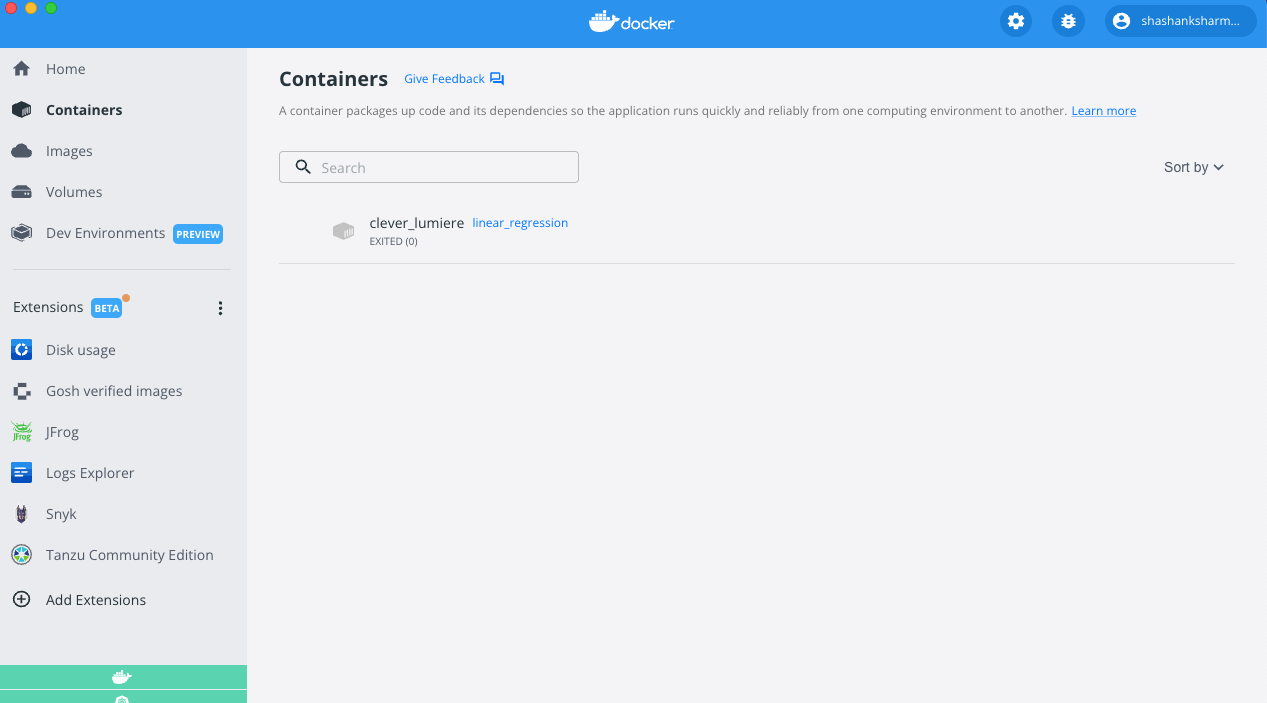
This command will create a container and execute the main.py script. Once we run the container, it’ll re-print the loss and estimates. The container will automatically exit after executing these commands. You can view your container’s status via Docker Desktop’s Container interface:

Desktop shows us that linear_regression executed the commands and exited successfully.

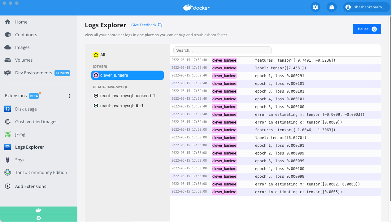
We can view our error estimates via the terminal or directly within Docker Desktop. I used a Docker Extension called Logs Explorer to view my container’s output (shown below):

Alternatively, you may also experiment using the Docker image that we created in this blog.

As we can see, the results from running the script on my system and inside the container are comparable.

To learn more about using containers with Python, visit these helpful links:

• Patrick Loeber’s talk, “How to Containerize Your Python Application with Docker”
• Docker documentation on building containers using Python

Want to learn more about PyTorch theories and examples?

We took a very tiny peek into the world of Python, PyTorch, and deep learning. However, many resources are available if you’re interested in learning more. Here are some great starting points:

• PyTorch tutorials
• Dive into Deep learning GitHub
• Machine Learning Mastery Tutorials

Additionally, endless free and paid courses exist on websites like YouTube, Udemy, Coursera, and others.

Stay tuned for more!

In this blog, we’ve introduced PyTorch and linear regression, and we’ve used the PyTorch framework to solve a very simple linear regression problem. We’ve also shown a very simple way to containerize your PyTorch application.

But, we have much, much more to discuss on deployment. Stay tuned for our follow-up blog — where we’ll tackle the ins and outs of deep-learning deployments! You won’t want to miss this one.